BGS 2019 Open Day activity: a taste of statistics from collecting data to making graphs

Sometimes people wonder what is behind the tables, graphs and models statisticians made. Are we playing tricks? Well, we cannot deny that we use some mathematical magic occasionally, but for most the time, it is about the data. To shed some light, we made a Shiny app in R, where we collect travel data from visitors to the BGS 2019 Open Day and produced some popular graphs using the data we collected live on the day. We also give a rough estimation of the carbon footprint of the journey!

Collecting Data

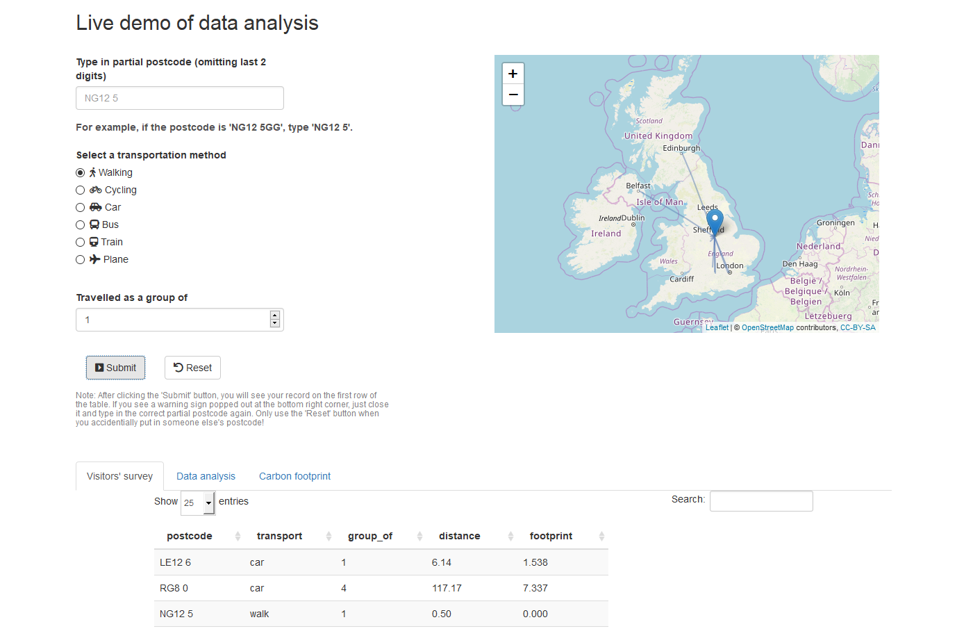
The app takes the partial post code of the visitors’ departure location, travel method (walking, cycling, driving, etc.) and travel group size as input. It first matches the partial post code with a spatial coordinate representing the ‘centre’ of the partial post code area. You can download the UK postcode table online. We used median longitude and latitude of all subareas within the partial post code area as the representative coordinate (fingers crossed that all post code areas are convex!). This gives the starting point. It then calculates the travel distance from the starting point to BGS Keyworth site for a particular transportation method using R package gmapsdistance. You may need to acquire Google map API key for this calculation. Finally, the app calculates the carbon footprint by multiplying the travel distance with a conversion factor (we used average figures for each transportation method from Wikipedia and some government documents), and that is everything we need to start the statistical analysis!

Making Graphs

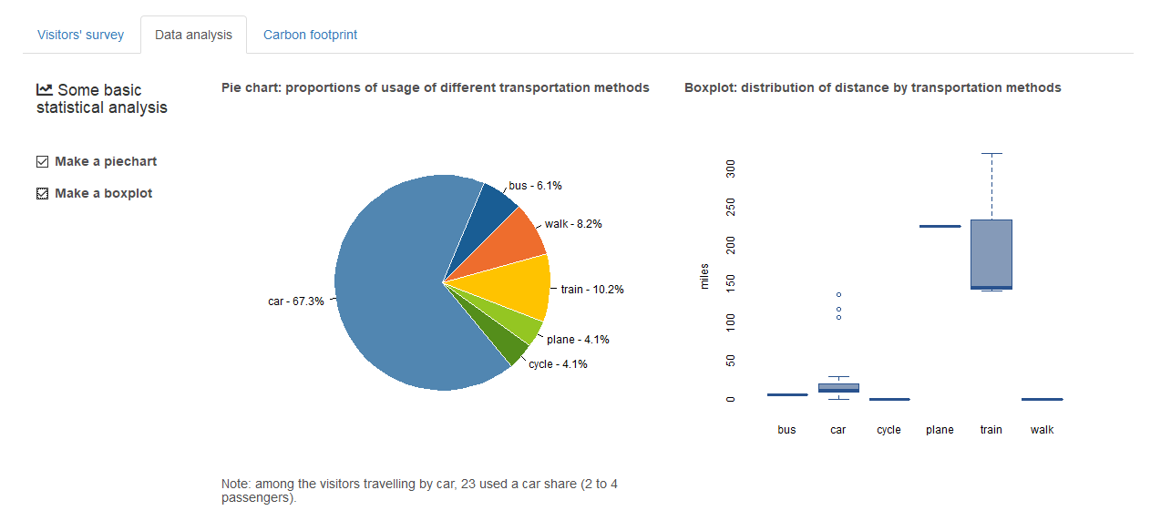
Using these information, we can make a pie chart showing the proportions of usage of each transportation method. That’s by summing up the 3rd column in the data table shown above using the 2nd column as a grouping factor. The pie chart in the screenshot below uses travel data from volunteers. Later that day we witnessed the proportion of car usage climbing up to over 80% as we factored in data from visitors. The good news is most of the visitors came sharing a car with their family and friends. We can make box plot of travel distances by different transportation method. Box plot is a nice way to visualise the variations of data in different groups.

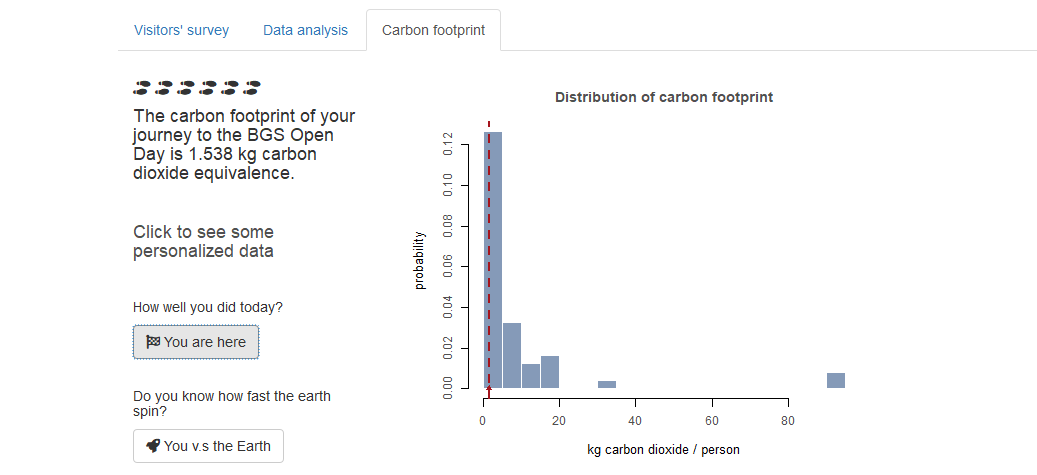
We can also make a histogram of the carbon footprints. To do that, we break the range of carbon footprints into several intervals and we count the number of observations falling into each interval. Here we convert the counts in each interval into probabilities, which makes it easy to investigate the distribution of the data. Modellers are often interested in whether the distribution is symmetric or right/left skewed, does it look like a normal distribution or a gamma distribution, etc. We have a pretty right skewed histogram here because there were BGS staff travelling from Belfast office by air (for volunteering), which resulted in those very large values.

Beyond the normal data

We used the app to demonstrate and collect some real data on the Open Day. You can also use it to investigate how these graphs change with ‘crazy’ input. For example, if you type in some data from your imaginary friend who cycled all the way from London to Keyworth, you would notice some dramatic change in the boxplot. It will hopefully give you some new insight into the meaning of these graphs and some idea on whether statisticians are playing tricks!

The complete Shiny UI and server scripts can be found following the link (https://github.com/GMY2018/FunStats2019) to GitHub.

A demonstrative version of the app can be accessed following the link (https://rapp-m.shinyapps.io/FunStats/) to Shinyapps.io.